Matrices are pretty confusing things, so here’s a quick summary of what they are, where they come from, and how you use them. Beware that matrices are very tricky, and require a lot of background knowledge before you can understand them in any depth.
Scalars are individual numbers – your age is a scalar, the length of an object is a scalar, and so on.
Some scalars:  .
.
Vectors are like lists of scalars, so a position in space is a vector – it consists of one scalar for each co-ordinate.
Some vectors: 
You can do algebra with vectors like you can with scalars. Addition is done by reading across the rows. For example:

And you can multiply a vector by a scalar:

You can even multiply two vectors together (their ‘dot product’) but you have to cheat a bit with the notation and write the firstone sideways, for reasons which will become clear when we look at matrices:

As vectors are made up of several scalars, you can think of matrices as being made up of several vectors. Consider a system of simultaneous equations:

Without explanation, here’s how you write that in matrix form:

What I’ve noticed is that every equation in the system had some number of  , some number of
  , and some number of
  . So, all you really need to describe the whole system is state what each of those coefficients is, and what each line was equal to. To understand what the matrix form means, look at the
  matrix a row at a time, as if it was a series of vector multiplications:


Which is the first equation of our system! Matrices aren’t just a quick way of writing down equations though – once you’ve got something into matrix form, there are a set of general operations you can perform on them to make finding a solution a lot less fiddly.
A matrix is like a 2D array of numbers. A matrix with  rows and
  columns is called a
  matrix. This is the other way round to the way you normally give co-ordinates, where the horizontal one is first and the vertical second. I think that’s just because you saw “rows and columns”, not “columns and rows”, and mathematicians wrote down the definition in words before drawing it out on paper.
If you want to give a matrix a name, the convention is to use a capital letter so you know it isn’t a scalar, which are always represented by lower-case letters.
You can add two matrices of the same size by adding the corresponding entries:

The same goes for subtracting matrices.
Multiplying matrices is a bit more involved. To multiply two matrices, first of all the second matrix has to have the same number of rows as the first matrix has columns. Multiplying an $m \times n$ matrix by an $n \times p$ matrix results in an $m \times p$ matrix.
To do the actual multiplication, start at the top-left entry of each matrix, and read right in the first matrix and down in the second matrix, summing up the products of each pair of entries as you go. That result is the value of the top-left entry of the result matrix.

Now go back and start again at the top-left of the first matrix, and the second entry in the top row of the second matrix, and proceed as before, to get the second entry of the top row. Once you’ve finished the top row, move down to the second row, of the first matrix, getting you the second row of the result, and so on and so forth. Very tedious work, but as long as you remember the order to do things in you can do it almost mechanically – read along the first matrix and down the second, then change row or column to get each entry in the result.
I don’t think anyone can get this right first time. If you ever really need to multiply two matrices, refer back here until you get a sensible answer. Unfortunately, matrix multiplication isn’t commutative, which means it matters which way round you do it. While $3 \times 7 = 7 \times 3 = 21$, the same isn’t always true for matrices:

but

That’s not even upside-down or reflected, it’s completely different numbers!
Though you can’t divide two matrices, so that’s one less thing to learn.
There are a few special matrices. First, the zero matrix:

is like the number zero – adding zero matrix to any other matrix leaves it as it is, and multiplying any matrix by the zero matrix results in the zero matrix. There’s a different zero matrix for every size, but you can always write it as just  without leading to any ambiguity.
Secondly, the identity matrix:

is like the number 1, with respect to multiplication. The identity matrix of any size is written as simply  Multiplying any matrix by an identity matrix (of the correct dimensions) leaves it as it is. You can also define the inverse of a square matrix
  as the matrix
  which, when multiplied by on either side, results in the identity matrix.
So, back to our system of simultaneous equations. If we find the inverse of the matrix on the left hand side of our equation, and multiply both sides by that, we are left with just  , so we can read off their values from the result of the right-hand side:

Nifty!
But this is deceptively simple, because finding the inverse of a matrix involves quite a bit of work. We’ll come back to this, after the last couple of matrix operations.
The transpose of a matrix is just the same matrix, written ‘sideways’ – rows become columns, and columns become rows. The transpose of a matrix is written  . So, reading down the first row of gives you the first column of , the second row gives the second column, and so on. Easy.
The determinant of a matrix is a bit like its size, but not really. It’s a scalar, but it can be negative or positive or even zero. What it really does is exactly what it says on the tin – it determine some of the characteristics of the matrix.
Now the determinant gets very complicated very quickly, so I’ll only go as far as telling you what it is for a matrix. First of all, the determinant of a  matrix is

(to show you’re working out the determinant of a matrix, write it in between straight lines instead of parentheses)
There are a few ways to work out the determinant of a matrix, but of course they all work out to the same number. The way I was taught was:
- Read along the top row.
- For each entry, cover up the row and column it belongs to, and work out the determinant of the matrix that is still visible, and multiply that number by the entry on the top row .
- Add the first and third results together and subtract the second one.

You can just remember that formula if you want, but I find it makes much more sense following the method.
Another way I’ve been taught is to start with  , and then “cycle round” the letters of each row, so you next add
  , and then
  . It’s horses for courses, really.
We’re almost there!
For each entry in a matrix, its minor is the determinant of the matrix made by deleting the row and column the original entry is in. The entry  of a matrix is even if
  is even, and odd if it is not. The cofactor of a matrix entry is the same as its minor in an even entry, or the opposite sign in an odd entry. You can form the matrix of cofactors for a matrix by setting each entry of the new matrix to be the cofactor of the entry in the old matrix.
Finally, the inverse of a matrix is the transpose of its matrix of cofactors, all divided by the determinant of the original matrix. Phew! Don’t worry, I have never succesfully remembered this. Look it up when you need it.

Clearly, if a matrix’s determinant is zero, you can’t divide by it, so it has no inverse. These matrices are called non-invertible matrices. Mathematicians do have a way with words!
So we can finally solve that system of equations! First, find the determinant:

That’s handy!
So, the matrix’s inverse is:

All that’s left to do is multiply both sides of the equation by this inverse (on the left, remember matrices aren’t commutative!)

We’re done! We can read off that  .
.
Now that was a huge amount of faff for something that you probably knew how to do when it was written as a set of simultaneous equations, but think about how you’d get a computer to do it that way. It would get very complicated, especially if you added more variables in. The matrix method, on the other hand, is very easy for a computer to do – it was just a series of well-defined mathematical operations, with no decisions to be made at any step.
But you almost never need to solve simultaneous equations in a game! What are some useful applications of matrices? Consider 2d transformations – moving, rotating and scaling. Moving and scaling are easy to do just with vectors, but what about rotation? Here’s how you do it with a set of scalar equations:

You can use the same trick as with the simultaneous equations before to write this in terms of matrices:

(I worked that matrix out by drawing a pair of axes and the graphs of sin and cos on paper, by the way. It’s another little thing it’s not worth trying to remember, but much more useful to work out each time you need it)
What this means is, you can work out the matrix for rotation by a particular angle once, and repeatedly apply that to a vector to rotate multiple times. It’s not obvious you can do that with the pair of equations above.If you find the inverse of a rotation matrix, you can also ‘undo’ a rotation very easily.
The matrix method gets vastly more useful when you move to 3d, and you end up with lots of equations and variables to keep track of.
So, that’s a brief summary of matrices. It’s a lot to learn in one go, and not at all intuitive. I think it’s best just to be aware of what they are, and refer back to this or somewhere like mathworld. Unless you’re doing a lot of 3d maths, I think you can get away with not knowing too much about them, as a games developer. Matrices also have all sorts of other applications, for example in graph theory and group theory, but I won’t bother covering those unless someone asks for it.
If you have any questions or don’t understand something, add a comment and I’ll endeavour to give satisfaction.
Read Full Post »


 , and an enemy at initial position
  moving in the direction
  .
. so that it collides with the enemy.
 .
. and
and  , then the bullet will move in parallel with the enemy, always staying the same distance from it.
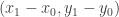 . The bullet can move along this line to collide with the bullet.
 frames to reach the bullet, we now get:
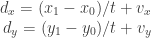

![\begin{array}{rcl} \left(\frac{1}{t}\right)^2 \left[ (x_1 - x_0)^2 + (y_1 - y_0)^2 \right] && \\ + \frac{1}{t} \left[ v_x (x_1 - x_0) + v_y ( y_1 - y_0) \right] &&\\ + v_x^2 + v_y^2 - V^2 &=& 0 \end{array}](https://s0.wp.com/latex.php?latex=%5Cbegin%7Barray%7D%7Brcl%7D+%5Cleft%28%5Cfrac%7B1%7D%7Bt%7D%5Cright%29%5E2+%5Cleft%5B+%28x_1+-+x_0%29%5E2+%2B+%28y_1+-+y_0%29%5E2+%5Cright%5D+%26%26+%5C%5C+%2B+%5Cfrac%7B1%7D%7Bt%7D+%5Cleft%5B+v_x+%28x_1+-+x_0%29+%2B+v_y+%28+y_1+-+y_0%29+%5Cright%5D+%26%26%5C%5C+%2B+v_x%5E2+%2B+v_y%5E2+-+V%5E2+%26%3D%26+0+%5Cend%7Barray%7D&bg=ffffff&fg=333333&s=0&c=20201002)
![\begin{array}{rcl} a &=& (x_1-x_0)^2 + (y_1-y_0)^2 \\ b &=& 2[ v_x(x_1-x_0) + v_y(y_1-y_0) ] \\ c &=& v_x^2 + v_y^2 - V^2 \end{array}](https://s0.wp.com/latex.php?latex=%5Cbegin%7Barray%7D%7Brcl%7D+a+%26%3D%26+%28x_1-x_0%29%5E2+%2B+%28y_1-y_0%29%5E2+%5C%5C+b+%26%3D%26++2%5B+v_x%28x_1-x_0%29+%2B+v_y%28y_1-y_0%29+%5D+%5C%5C+c+%26%3D%26++v_x%5E2+%2B+v_y%5E2+-+V%5E2+%5Cend%7Barray%7D&bg=ffffff&fg=333333&s=0&c=20201002)

 and
and  , and you’re done!